Getting The Sumif Date Range To Work

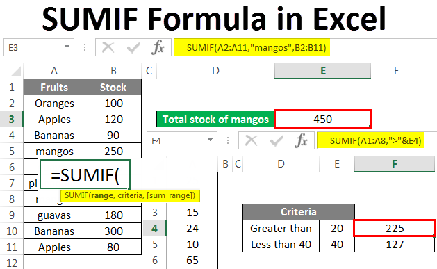
You utilize the SUMIF function to sum the worths in a variety that satisfy standards that you specify. For instance, mean that in a column which contains numbers, you desire to sum just the values that are bigger than 5. You can utilize the following formula: =SUMIF(B 2: B 25,"> 5") This video clip becomes part of a training course called Include numbers in Excel.

As an example, the formula =SUMIF(B 2: B 5, "John", C 2: C 5) amounts only the worths in the array C 2: C 5, where the matching cells in the variety B 2: B 5 equal "John." To sum cells based upon multiple criteria, see SUMIFS function. SUMIF(range, requirements, [sum_range] The SUMIF function phrase structure has the adhering to debates: range Required.

Cells in each range need to be numbers or names, varieties, or referrals that include numbers. Space as well as message worths are overlooked. The chosen range may have days in conventional Excel format (examples below). criteria Called for. The standards in the kind of a number, expression, a cell referral, message, or a function that specifies which cells will certainly be added.

Essential: Any message criteria or any type of requirements that includes logical or mathematical icons should be enclosed in dual quotation marks ("). If the criteria is numerical, double quotation marks are not needed. sum_range Optional. The actual cells to include, if you want to add cells besides those specified in the variety debate.

How Sumif Vlookup can Save You Time, Stress, and Money.

You can make use of the wildcard personalities-- the concern mark (?) and also asterisk (*)-- as the requirements disagreement. An enigma matches any type of single character; an asterisk matches any kind of sequence of characters. If you wish to find an actual question mark or asterisk, type a tilde (~) coming before the character. The SUMIF function returns wrong outcomes when you utilize it to match strings longer than 255 personalities or to the string #VALUE!.

The actual cells that are added are figured out by utilizing the upper leftmost cell in the sum_range disagreement as the start cell, and afterwards including cells that match in dimension and also shape to the range disagreement. As an example: If range is And sum_range is Then the actual cells are A 1: A 5 B 1: B 5 B 1: B 5 A 1: A 5 B 1: B 3 B 1: B 5 A 1: B 4 C 1:D 4 C 1:D 4 A 1: B 4 C 1: C 2 C 1:D 4 However, when the range and sum_range disagreements in the SUMIF feature do not include the very same variety of cells, worksheet recalculation might take longer than expected.

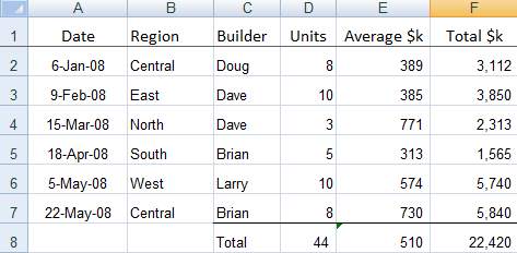
For solutions to show results, pick them, press F 2, as well as after that press Enter. If you require to, you can adjust the column sizes to see all the information. Property Worth Commission Data $100,000 $7,000 $250,000 $200,000 $14,000 $300,000 $21,000 $400,000 $28,000 Formula Description Result =SUMIF(A 2: A 5,"> 160000", B 2: B 5) Sum of the payments for residential property values over $160,000.

$900,000 =SUMIF(A 2: A 5,300000, B 2: B 5) Amount of the commissions for residential property worths equal to $300,000. $21,000 =SUMIF(A 2: A 5,">" & C 2, B 2: B 5) Sum of the commissions for home worths higher than the value in C 2. $49,000 Instance 2 Replicate the example information in the following table, and also paste it in cell A 1 of a brand-new Excel worksheet.

8 Easy Facts About Sumif Vlookup Explained

If you need to, you can change the column sizes to see all the data. Category Food Sales Vegetables Tomatoes $2,300 Veggies Celery $5,500 Fruits Oranges $800 Butter $400 Veggies Carrots $4,200 Fruits Apples $1,200 Formula Summary Result =SUMIF(A 2: A 7,"Fruits", C 2: C 7) Sum of the sales of all foods in the "Fruits" category.

$12,000 =SUMIF(B 2: B 7,"* es", C 2: C 7) Sum of the sales of all foods that end in "es" (Tomatoes, Oranges, as well as Apples). $4,300 =SUMIF(A 2: A 7,"", C 2: C 7) Amount of the sales of all foods that do not have actually a category specified. $400 Top of Web page You can constantly ask an expert in the Excel User Voice.

To sum if cells consist of certain text, you can use the SUMIF feature with a wildcard. In the instance revealed, cell G 6 contains this formula: =SUMIF(C 5: C 11,"* tee shirt *", D 5:D 11) This formula amounts the quantities in ... To subtotal data by team or label, straight in a table, you can make use of a formula based on the SUMIF feature.

To sum if higher than, you can make use of the SUMIF feature. In the instance revealed, cell H 6 has this formula: =SUMIF(amount,"> 1000") where "amount" is a called array for cells D 5:D 11. This formula sums ... To allow a dropdown with an "all" option you can make use of data validation for the dropdown checklist, and also a formula based on IF, AMOUNT, and also SUMIF functions to compute a conditional amount.

Top Guidelines Of Sumif Multiple Columns

To sum if cells end with details message, you can utilize the SUMIF feature. In the example shown, cell G 6 includes this formula: =SUMIF(product,"* hat", quantity) This formula amounts cells in the named range quantity (D 5: ... If you require to subtotal numbers by shade, you can easily do so with the SUMIF feature.

To sum if cells include certain text in one more cell, you can use the SUMIF function with a wildcard and also concatenation. In the example shown, cell G 6 includes this formula: =SUMIF(C 5: C 11,"*"& F 6 & ... To sum numbers based on other cells amounting to either one worth or one more (either x or y), you can utilize the SUMIF function.

The ... To conditionally sum identical arrays that exist in separate worksheets, done in one formula, you can do so with the SUMIF function + INDIRECT, covered in SUMPRODUCT. In the instance, the formula appears like this: =... If you need to sum worths when cells are equal to one of lots of points, you can use a formula based upon the SUMIF and SUMPRODUCT functions.

sumif excel array formula sumif excel vba programming sumif excel with index match